Discounted expectations
After our little detour into GARCHery, we’re back to discuss capital market expectations. In Mean expectations, we examined using the historical average return to set return expectations when constructing a portfolio. We noted hurdles to this approach due to factors like non-normal distributions, serial correlation, and ultra-wide confidence intervals.
While we highlighted these obstacles and offered a few suggestions to counteract such drawbacks, on first blush it didn’t seem like historical averages were all that satisfactory. But all is not lost! There are other methods to estimating expected returns; namely, discounted cash flow (DCF) and risk premia. In this post, we’ll discuss the first, DCF.
The intuition behind using a DCF is that any cash-generating asset should equal the present value of its future cash flows. If it doesn’t, there might be a market inefficiency. But forgetting about that for a second, it suggests that if you can estimate the cash flows well enough, you can calculate the expected return. How do you do that? Using a modified Gordon Growth Model.
The original Gordon Growth Model was based on dividends and essentially said the price today of a stock is equal to next year’s dividend divided by the discount rate less the growth rate in dividends. This equates to:
\[V_{t_{0}} = \frac{D_{t_{1}}}{(r - g)}\]
Where V = value, D = dividend, r = discount rate, g = growth rate, and t0 and t1 = time periods
The equation assumes a constant growth in dividends. Any type of cash can be substituted for dividends, allowing the equation to be applied to almost any asset that generates or returns cash to holders. Thus, substituting cash flow for dividends and rearranging the terms, one can solve for return, which is often called “required return” in that it is the return required to make the cash flows equal to the current value. The formula becomes:
\[r = \frac{CF_{t_{1}}}{V_{t0}} + g\]
Where CF = cash flow
Of course, the equation can get even more complicated with multi-period cash flows and different discount rates. But we’ll keep it simple for now. To calculate the required return, all we need to do is figure out the growth rate. For the S&P 500, our preferred index for analysis, figure out what the long-run growth rate of cash flow will be and then you’ve got the expected return. Simple!
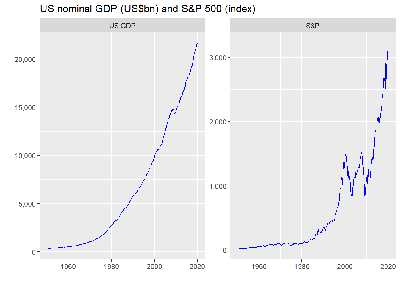
But plugging in the growth rate assumes you know what future cash flows will be. And how the heck do you forecast that? If you’re an equity analyst, that’s what you spend a lot of your time doing. But even the best of the best are probably right as often as a tipsy dart champion. To circumvent that, one solution is to assume that, in aggregate, cash flow grows at the nominal growth rate of the economy. Why should this work well for stocks in aggregate? Because the market shouldn’t grow much beyond the economy over the long run. Using GDP also helps smooth out the bumps, since the GDP growth rate has been pretty stable over time. That is easy enough to see in the chart below.
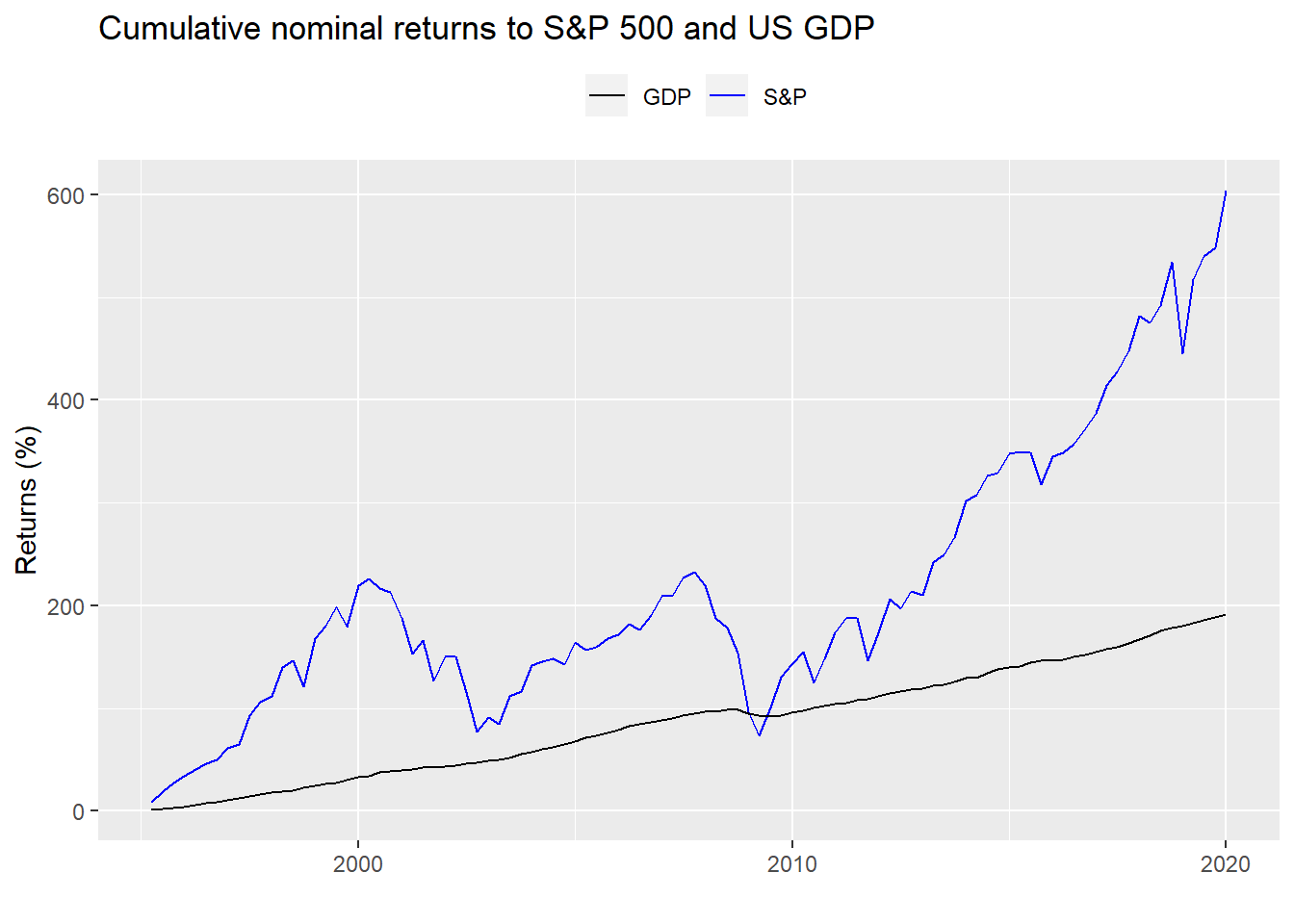
Graphing a comparison in cumulative returns, seems to support the GDP workaround, at least until the mid-1990s.
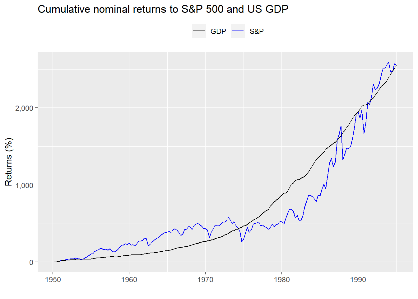
After that, cumulative growth starts to diverge.
If that chart doesn’t look like a poster child for overvalued, we don’t know what does! But that’s not the point of this post. We’re trying to estimate expected returns using a DCF. Hence, we’ll explore the concept using the S&P and then assess how accurate a DCF is.
First, we calculate the average quarter-over-quarter return of the S&P 500 and the nominal growth rate of US GDP. As one can see, since 1950 they’re pretty close.
| GDP | S&P 500 |
|---|---|
| 6.4 | 7.8 |
Indeed, when we run a test for the difference in means we find the p-value is 0.5, suggesting any difference is likely due to randomness. Thus, it seems legitimate on some very rough analysis to use nominal GDP growth as a proxy for cash flow growth.
To get the expected return, one just needs to add the first component of the re-arranged equation above (e.g. CF/V), which is next year’s current yield1 to the growth rate and you’re done. In the case of stocks, that current yield is frequently the dividend yield, but it can be free cash flow yield or a number of metrics, which we’ll briefly mention below. In any case, if GDP grows around 6% and the median dividend yield of the S&P has been around 2%, then it’s relatively easy to see why the rule-of-thumb expected return is around 7-9%.
But how well does this actually work in reality? If we’re going to use nominal GDP as a proxy for cash, it should be a relatively good predictor. So we’ll need to build a model to test the predictive power of GDP. We’ll also need a way to compare our GDP model against a benchmark.To do this, we’ll start with a naive model, which will simply forecast the next period of growth as equal to the prior period. We’ll then compare the accuracy of other models with the naive model. We’ll look at the periods before and after 1995 and use the root mean squared error (RMSE) as the accuracy statistic.
First, we show the naive model’s accuracy. That is, we compare the current period return vs the prior period, assuming the current period will be close to the prior. No fancy regressions here! Just assume the future looks like the past. Using those two figures we calculate the RMSE. Then, we scale the RMSE by the average of actual results to give one a sense of the size of the error.
| Period | RMSE | Scaled |
|---|---|---|
| Pre | 0.10 | 5.58 |
| Post | 0.11 | 5.62 |
As one can see there is little difference between pre- and post-1995 accuracy, as would be expected since there really isn’t much opportunity for overfitting. Additionally, the RMSE is over 5x the average, which is pretty high.
Now, let’s compare the naive model to our first model in which we assume the next period’s return is the same as the prior period GDP growth rate. One note on methodology: for this and all proceeding models, since there are a number of revisions and the final GDP figures aren’t reported until near the end of the next quarter, the model will effectively use GDP lagged by two quarters to forecast the next period’s return. For example, the final GDP estimate for the the third quarter is typically not published until near the end of the fourth quarter. Thus, to forecast the first quarter’s return for the following year, we’d use the third quarter GDP growth rate. If we didn’t adjust the data, the model would suffer look-ahead bias.2
We’ll show the comparisons going forward graphically to make it a bit easier to see.
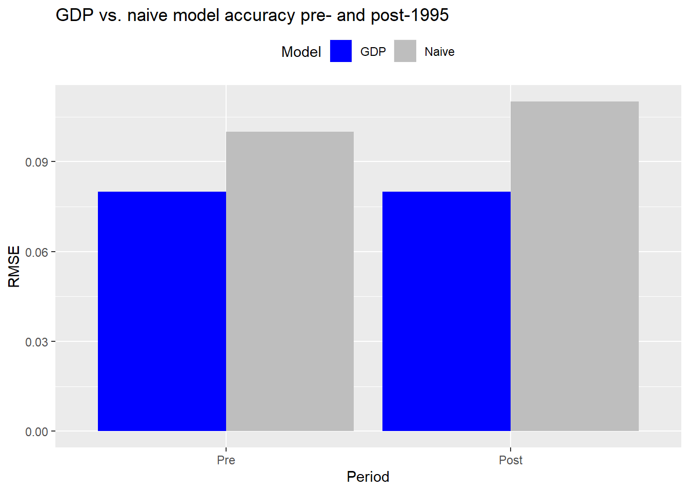
Interesting! The GDP model performs better than the naive model both pre- and post-1995 (the RMSE is shorter). Additionally, while the naive model performs slightly worse post-1995 vs pre, the GDP model seems about the same for both periods.
This is all just a warm-up to get some basic models going. Unless we’re turning over the portfolio every quarter3, our focus should be on returns over a year or few years. Let’s conduct the same analysis, but look at the next four quarters’ cumulative return on a rolling basis. As before, we’ll use the naive model, which in this case will use the prior four quarters to forecast the next four quarters’ cumulative return. We’ll then apply that same methodology to nominal GDP. As with the prior model, the closest GDP figure will be on a two quarter lag.
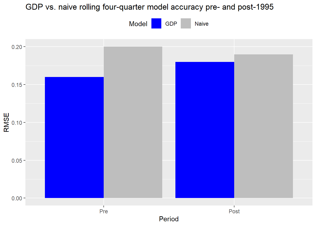
Accuracy declines for the GDP in the post-1995 period vs. pre-95. Yet, the GDP model still performs better than the naive model in both periods. That the naive model performs slightly better in the post-1995 period might be due to stronger serial correlation in that period, but we’ll have to examine that another time.
We could keep going like this, adding more look-back and look-forward periods. But it is starting to get a bit repetitive. So let’s jump to a model that takes the rolling cumulative average return for the entire period and then assumes that will be the average annual return for the next three years. While this might seem a bit arbitrary, it is meant to capture the original intuition that the long-run average nominal GDP growth rate is a good proxy for the cash flow growth rate. The three-year look forward is also the period many longer term focused investors use when setting return expectations.
As before, we’ll calculate the root mean squared error over the period of interest. But in this case, the post-1995 RMSE will feature “memory” for all of the prior history. The only difference in the time series vs. the prior models is that we begin in 1960 so that we have a stable enough average for historical annualized returns at the beginning of the series.
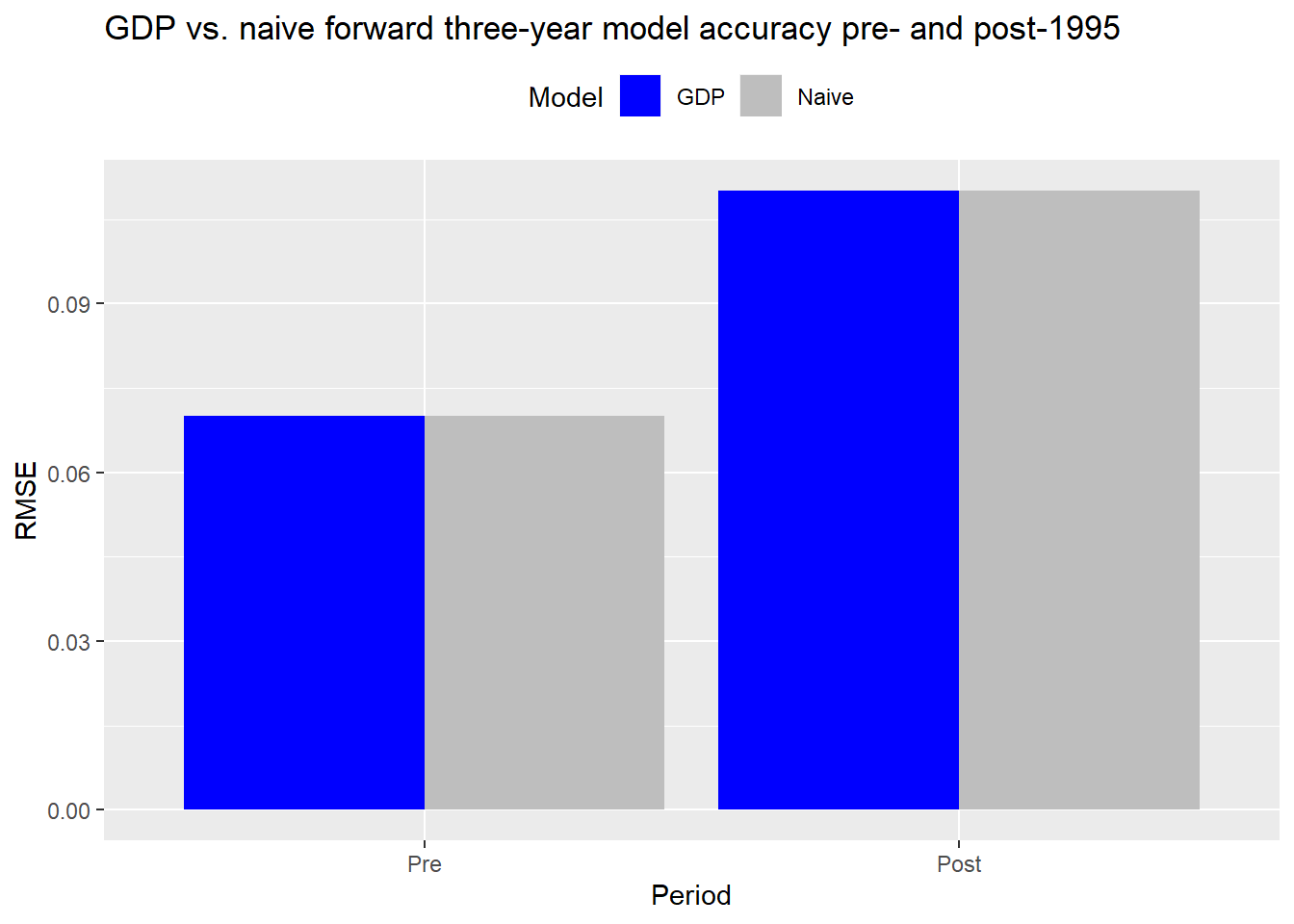
The graph above is not a joke. The GDP and naive models yield very similar accuracy on the longer term data. With rounding, they’re virtually the same. This confirms the intuition that over the long-run the S&P growth rate does approximate nominal GDP. But if that’s the case, why not just use the historical average return? It’s certainly less effort. While that might work for the S&P, there is no guarantee it will work for other indices, sectors, or even individual stocks.
Let’s sum up our findings. Using a DCF to set expected returns appeals to the intuition that an asset is worth the net present value of its future cash flows. Hence, if you have a good estimate of an asset’s cash flow growth rate, you’ll be able to back into the required return, which should be the future yield plus the growth rate. Forecasting the growth rate is not that easy, so one recommendation is to use the nominal growth rate of the economy as a proxy for the cash flow rate. This seems reasonable if you’re applying it to an asset class like stocks. It probably doesn’t work quite so well (or at all) for other asset classes, but we’ll shelve that discussion for another time.
To test how well GDP growth is able to describe price returns to the S&P, we compared various GDP models with similar naive models using different aggregation periods. Over some aggregation periods, the GDP model performed better than the naive. However, over the long run, the two models generated virtually the same accuracy. This begs the question why use nominal GDP growth rates as a proxy for cash flow growth rates at all? While it may be similar to the historical average, on shorter timeframes GDP works better. Additionally, for indices with shorter histories, or more volatility (e.g. emerging markets), using a GDP-based DCF is a reasonable alternative.
Interestingly, our intention was not to pit the historical mean method against the DCF at the outset of this post, but that is what seems to fall out, at least for the S&P. We’d of course need to test this on other developed markets. This doesn’t, however, invalidate the DCF method.
On asset classes where cash flow is not as correlated with the overall economy, a DCF method would likely outperform the historical average. Additionally, within asset classes—for example, small cap value vs. large cap growth—using a DCF could yield better forecasts than the historical mean. But in these cases, the DCF would likely be derived using data other than GDP, since returns would probably be more idiosyncratic. If asset selection is even more granular—say at the company level—then a DCF is much more appropriate, assuming the analyst has insight into the company and/or industry.
While we didn’t go into detail about what may have caused the apparent regime change pre and post-1995, we address a work around for that briefly in the Appendix below.
In our next post, we’ll examine risk premia as the third method for setting capital market expectations. Until then, the code, following the appendix, is below.
Appendix
As we showed in the cumulative return chart above, the S&P looks like its growth has become unhinged from GDP. One way to explain that is by expanding the DCF model to include buybacks and changes in price-to-earnings multiples. That is, if buybacks are increasing, then more cash is being returned to shareholders, which equates to value that can be employed at higher returns. Changes in multiples drive returns if the market is willing to pay more for the same amount of earnings due to perceived lower risk or lower interest rate levels in the economy. Thus, as buybacks and multiples have increased over past decade, returns to the S&P have disconnected from GDP.
While adding such nuances may be great way to explain changes in the historical rate of return, applying them prospectively is tough due to the difficulty in forecasting multiple expansion or buyback policies. If you’d like more details on this methodology see the Grinold-Kroner Model.
A way to correct for the divergence without getting too far afield into factors that are difficult to forecast would be to transform the data somehow. One way would to be take the logs of the underlying values of both time series to account for different rates. We show this in the graph below. Note we adjusted GDP down an order of magnitude to make the line scale better with the S&P.
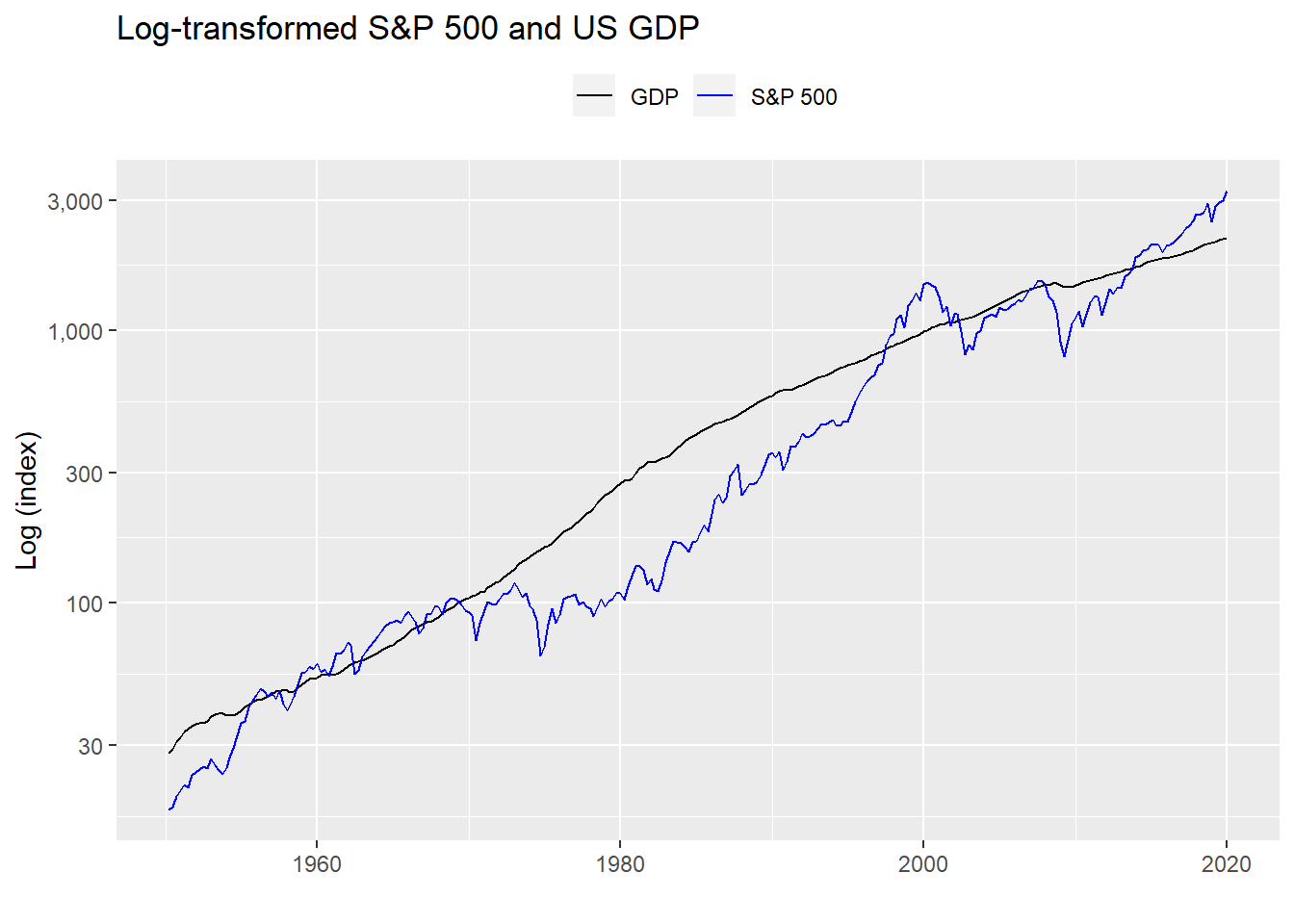
That transformation looks good and we haven’t tortured the data too much. The question is how accurately would nominal GDP forecast the S&P? When we regress the log-transformed level of the S&P vs. the log-transformed nominal GDP on the pre-1995 data, we find the output below.
| Term | Estimate | Statistic |
|---|---|---|
| Log(Intercept) | -0.9 | -5.7 |
| Log(GDP) | 0.8 | 36.5 |
The estimates are statistically significant and the model explains almost 88% of the variability in the S&P. But the proof is in the accuracy on out-of-sample data, which we show below.
| Period | RMSE | Scaled |
|---|---|---|
| Pre | 43.47 | 0.32 |
| Post | 1028.23 | 0.71 |
Accuracy takes a big hit on the out-of-sample data, plummeting by two orders of magnitude. That said, out-of-sample scaled accuracy isn’t quite so bad, though still double the in sample. To estimate the expected return we’d need to chug through a few more calculations, which wouldn’t be onerous. But now we’d be forecasting the level of GDP, which wouldn’t be difficult if we simply used a steady state growth rate. But then why go through all that if accuracy declines so much in the first place? If you have a strong opinion on that, shoot us an email to the address after the code. Speaking of code, here it is.
## Load packages
suppressPackageStartupMessages({
  library(tidyquant)
  library(tidyverse)
})

# Load data
sp <- getSymbols("^GSPC", src = "yahoo", from = "1950-01-01", to = "2020-01-01",
                 auto.assign = FALSE) %>%
  Ad() %>%
  `colnames<-`("sp")

sp_qtr <- to.quarterly(sp, indexAt = "lastof", OHLC = FALSE)

## GDP data comes in as of the first day of the quarter, but that isn't how it's reported
## Need to align it at least so that it's current with end of the quarter S&P data
gdp <- getSymbols("GDP", src = "FRED", from = "1950-01-01", to = "2020-01-01",
                  auto.assign = FALSE) %>%
  `colnames<-`("gdp")

qtr <- index(to.quarterly(sp["1950/2019"], indexAt = "lastof", OHLC = FALSE))
gdp_eop <- xts(coredata(gdp["1950/2019"]), order.by = qtr) # change to end-of-period

merged <- merge(sp_qtr, gdp_eop)

df <- data.frame(date = index(merged), coredata(merged)) %>%
  mutate(sp_ret = c(0, diff(log(sp))),
         gdp_ret = c(0,diff(log(gdp))))

## Dual chart
df %>%
  gather(key, value, -date) %>%
  filter(key %in% c("sp", "gdp")) %>%
  ggplot(aes(date, value)) +
  geom_line(color = "blue") +
  scale_y_continuous(labels = scales::comma)+
  facet_wrap(~key, scales = "free_y", labeller = as_labeller(c("sp" = "S&P",
                                                               "gdp" = "US GDP"))) +
  labs(x = "",
       y = "",
       title = "S&P 500 and US GDP nominal values")

## Cumulative return chart
df %>%
  filter(date < "1995-01-01") %>%
  mutate_at(vars("sp_ret", "gdp_ret"), function(x) cumprod(1+(exp(x)-1))-1) %>%
  ggplot(aes(x =date)) +
  geom_line(aes(y = sp_ret*100, color = "S&P")) +
  geom_line(aes(y = gdp_ret*100, color = "GDP")) +
  scale_color_manual("", values = c("black", "blue")) +
  scale_y_continuous(labels = scales::comma)+
  labs(x="",
       y = "Returns (%)",
       title = "Cumulative nominal returns to S&P 500 and US GDP") +
  theme(legend.position = "top")

## Cumulative return chart
df %>%
  filter(date >= "1995-01-01") %>%
  mutate_at(vars("sp_ret", "gdp_ret"), function(x) cumprod(1+(exp(x)-1))-1) %>%
  ggplot(aes(x =date)) +
  geom_line(aes(y = sp_ret*100, color = "S&P")) +
  geom_line(aes(y = gdp_ret*100, color = "GDP")) +
  scale_color_manual("", values = c("black", "blue")) +
  scale_y_continuous(labels = scales::comma)+
  labs(x="",
       y = "Returns (%)",
       title = "Cumulative nominal returns to S&P 500 and US GDP") +
  theme(legend.position = "top")

## Return comparisons
df %>%
  summarise_at(vars("gdp_ret", "sp_ret"),
               function(x) round(exp(mean(x, na.rm = TRUE)*4)-1, 3)*100) %>%
  rename("GDP" = gdp_ret,
         "S&P 500" = sp_ret) %>%
  knitr::kable(caption = "Average annualized growth rates (%)")


t_test <- round(t.test(df$gdp_ret, df$sp_ret)$p.value,2)

## Naive model
train_naive <- df %>%
  filter(date < "1995-01-01")

test_naive <- df %>%
  filter(date >= "1995-01-01")

rmse_in_naive <- sqrt(mean((train_naive$sp_ret - lag(train_naive$sp_ret))^2, na.rm = TRUE))
rmse_out_naive <- sqrt(mean((test_naive$sp_ret - lag(test_naive$sp_ret))^2, na.rm = TRUE))

scale_in_maive <- rmse_in_naive/mean(train_naive$sp_ret, na.rm = TRUE)
scale_out_maive <- rmse_out_naive/mean(test_naive$sp_ret, na.rm = TRUE)

data.frame(Period = c("Pre", "Post"),
           RMSE = c(rmse_in_naive, rmse_out_naive),
           Scaled = c(scale_in_maive, scale_out_maive)) %>%
  mutate_at(vars(-"Period"),round, 2) %>%
  knitr::kable(caption = "Naive model accuracy pre- and post-1995")

# GDP model
df_lag <- df %>%
  mutate(gdp_lag = lag(gdp,2)) %>%
  mutate(gdp_lag_ret = c(NA,diff(log(gdp_lag))))

train_gdp <- df_lag %>%
  filter(date < "1995-01-01")

test_gdp <- df_lag %>%
  filter(date >= "1995-01-01")

rmse_in_gdp <- sqrt(mean((train_gdp$sp_ret - train_gdp$gdp_lag_ret)^2, na.rm = TRUE))
rmse_out_gdp <- sqrt(mean((test_gdp$sp_ret - test_gdp$gdp_lag_ret)^2, na.rm = TRUE))


data.frame(Model = c("Naive", "Naive", "GDP", "GDP"),
           Period = factor(c("Pre", "Post","Pre", "Post"), levels = c("Pre", "Post")),
           RMSE = c(rmse_in_naive, rmse_out_naive, rmse_in_gdp, rmse_out_gdp),
           Scaled = c(scale_in_maive, scale_out_maive, scale_in_gdp, scale_out_gdp)) %>%
  mutate_at(vars(-c("Period","Model")),round, 2) %>%
  gather(key, value, -c(Model, Period)) %>%
  filter(key == "RMSE") %>%
  ggplot(aes(Period, value, fill = Model)) +
  geom_bar(stat = "identity", position = "dodge")+
  labs(y = "RMSE",
       title = "Model accuracy comparison pre- and post-1995") +
  scale_fill_manual(values = c("blue", "grey")) +
  theme(legend.position = "top")


## Naive hist model
df_for <- df_lag %>%
  mutate(sp_lead = rollapply(sp_ret, 4, sum, align = 'left', fill = NA),
         sp_lag = rollapply(sp_ret, 4, sum, align = "right", fill = NA))

train_naive_hist <- df_for %>%
  filter(date < "1995-01-01")

test_naive_hist <- df_for %>%
  filter(date >= "1995-01-01")

rmse_in_naive_hist <- sqrt(mean((train_naive_hist$sp_lead - train_naive_hist$sp_lag)^2, na.rm = TRUE))

rmse_out_naive_hist <- sqrt(mean((test_naive_hist$sp_lead - test_naive_hist$sp_lag)^2, na.rm = TRUE))

## GDP1 model
df_lag1 <- df_lag %>%
  mutate(sp_lead = rollapply(sp_ret, 4, sum, align = 'left', fill = NA),
         gdp_lag_yr = rollapply(gdp_lag_ret, 4, sum, align = 'right', fill = NA))

train_gdp1 <- df_lag1 %>%
  filter(date < "1995-01-01")

test_gdp1 <- df_lag1 %>%
  filter(date >= "1995-01-01")

rmse_in_gdp1 <- sqrt(mean((train_gdp1$sp_lead - train_gdp1$gdp_lag_yr)^2, na.rm = TRUE))

rmse_out_gdp1 <- sqrt(mean((test_gdp1$sp_lead - test_gdp1$gdp_lag_yr)^2, na.rm = TRUE))

data.frame(Model = c("Naive", "Naive", "GDP", "GDP"),
           Period = factor(c("Pre", "Post","Pre", "Post"), levels = c("Pre", "Post")),
           RMSE = c(rmse_in_naive_hist, rmse_out_naive_hist, rmse_in_gdp1, rmse_out_gdp1)
           ) %>%
  mutate_at(vars(-c("Period","Model")),round, 2) %>%
  gather(key, value, -c(Model, Period)) %>%
  filter(key == "RMSE") %>%
  ggplot(aes(Period, value, fill = Model)) +
  geom_bar(stat = "identity", position = "dodge")+
  labs(y = "RMSE",
       title = "Model accuracy comparison") +
  scale_fill_manual(values = c("blue", "grey")) +
  theme(legend.position = "top")

## Naive all hist model
df_naive_hist_all <- df %>%
  mutate(sp_lead = rollapply(sp_ret, 12, function(x) sum(x)/3, align = 'left', fill = NA),
         sp_lag = rollapply(sp_ret, 4, sum, align = 'right', fill = NA),
         sp_cummean = cummean(ifelse(is.na(sp_lag), 0, sp_lag)))

train_naive_hist_all <- df_naive_hist_all %>%
   filter(date >= "1960-01-01")

rows <- nrow(train_naive_hist_all)

rmse_pre_naive_hist_all <- sqrt(mean((train_naive_hist_all$sp_lead[1:140] -
                                        train_naive_hist_all$sp_cummean[1:140])^2, na.rm = TRUE))

rmse_post_naive_hist_all <- sqrt(mean((train_naive_hist_all$sp_lead[141:rows] -
                                         train_naive_hist_all$sp_cummean[141:rows])^2,
                                      na.rm = TRUE))

## GDP2 model
df_lag2 <- df_lag %>%
  mutate(sp_lead = rollapply(sp_ret, 12, function(x) sum(x)/3, align = 'left', fill = NA),
         gdp_lag_yr = rollapply(gdp_lag_ret, 4, sum, align = 'right', fill = NA),
         gdp_cummean = cummean(ifelse(is.na(gdp_lag_yr), 0, gdp_lag_yr)))

train_gdp2 <- df_lag2 %>%
  filter(date >= "1960-01-01")

rows_gdp <- nrow(train_gdp2)
rmse_pre_gdp2 <- sqrt(mean((train_gdp2$sp_lead[1:140] - train_gdp2$gdp_cummean[1:140])^2, na.rm = TRUE))

rmse_post_gdp2 <- sqrt(mean((train_gdp2$sp_lead[141:rows_gdp] -
                               train_gdp2$gdp_cummean[141:rows_gdp])^2,
                            na.rm = TRUE))

data.frame(Model = c("Naive", "Naive", "GDP", "GDP"),
           Period = factor(c("Pre", "Post","Pre", "Post"), levels = c("Pre", "Post")),
           RMSE = c(rmse_pre_naive_hist_all, rmse_post_naive_hist_all,
                    rmse_pre_gdp2, rmse_post_gdp2)) %>%
  mutate_at(vars(-c("Period","Model")),round, 2) %>%
  knitr::kable(caption = "Naive model accuracy")

data.frame(Model = c("Naive", "Naive", "GDP", "GDP"),
           Period = factor(c("Pre", "Post","Pre", "Post"), levels = c("Pre", "Post")),
           RMSE = c(rmse_pre_naive_hist_all, rmse_post_naive_hist_all,
                    rmse_pre_gdp2, rmse_post_gdp2)) %>%
  mutate_at(vars(-c("Period","Model")),round, 2) %>%
  ggplot(aes(Period, RMSE, fill = Model)) +
  geom_bar(stat = "identity", position = "dodge")+
  labs(y = "RMSE",
       title = "Model accuracy comparison pre and post 1995") +
  scale_fill_manual(values = c("blue", "grey")) +
  theme(legend.position = "top")

df %>%
  mutate(gdp = gdp/10) %>%
  gather(key, value, -date) %>%
  filter(key %in% c("sp", "gdp")) %>%
  ggplot(aes(date,value, color = key)) +
  geom_line() +
  scale_y_log10(labels = scales::comma) +
  scale_color_manual("", labels = c("GDP", "S&P 500"),
                     values = c("black", "blue")) +
  labs(x="",
       y = "Log (index)",
       title = "Cumulative nominal log returns to S&P 500 and US GDP") +
  theme(legend.position = "top")

## Log model
train_log_mod <- lm(log(sp) ~ log(gdp_lag), train_gdp)
in_log <- predict(train_log_mod, train_gdp)
rmse_in_log <- sqrt(mean((train_gdp$sp - exp(in_log))^2, na.rm = TRUE))

out_log <- predict(train_log_mod, test_gdp)
rmse_out_log <- sqrt(mean((test_gdp$sp - exp(out_log))^2, na.rm = TRUE))

# Coeffiecients
broom::tidy(train_log_mod) %>%
  select(term, estimate, statistic) %>%
  mutate_at(vars(-"term"), round, 1) %>%
  mutate(term = ifelse(term == '(Intercept)', "Intercept", "Log of GDP")) %>%
  rename("Term" = term,
         "Estimate" = estimate,
         "Statistic" = statistic) %>%
  knitr::kable()

# R-squared
rsq <- broom::glance(train_log_mod)$r.squared %>% round(.,2)*100

scale_in_log <- rmse_in_log/mean(train_gdp$sp, na.rm = TRUE)
scale_out_log <- rmse_out_log/mean(test_gdp$sp, na.rm = TRUE)

data.frame(Period = c("Pre", "Post"),
           RMSE = c(rmse_in_log, rmse_out_log),
           Scaled = c(scale_in_log, scale_out_log)) %>%
  mutate_at(vars(-"Period"),round, 2) %>%
  knitr::kable(caption = "Log model accuracy pre- and post-1995")
In effect, cash that will be returned or attributed to the owner of the asset.↩
Indeed, while we correct for look-ahead bias, we introduce a different bias: one of stale data. The market will already have discounted future cash flows based on Advance estimates and revisions. Unfortunately, getting the Advance figures is not so easy! However, as the next models rely on a longer time frame, we hope we’ve removed some of that bias.↩
Which happens for most active managers whose turnover rate is almost 90%, according to Morningstar.↩